Open problems in intercurrent-event handling and missing-data mechanisms in randomised clinical trials

A simulation-based assessment of the regulatory toolkit

Márton Kiss M.D. (https://martonkissdr.hu/)

2026-06-12

Contents

• Part 1 — A short history — how we got from LOCF to the estimand framework
• Part 2 — Generating the data — one MADRS depression trial, simulated so we know the truth
• Part 3 — How the data go missing — MCAR / MAR / MNAR, and what selection does to the analysis
• Part 4 — The reference-based toolkit — five macros, five estimands, the δ convention
• Part 5 — Operating characteristics — coverage, the two variance camps, and the regret
• Part 6 — The tipping point — how far from MAR before the result flips?

What this talk is about

• Aim: we run a longitudinal depression trial, measured on the MADRS scale across ten weeks, and — as in every real trial — some patients stop coming. We want the week-10 treatment effect, but the patients who left we can no longer measure.
• The clinician’s questions are blunt: does the drug lower MADRS more than placebo, and how far does that answer depend on assumptions about the people we never finished following?
• This is the territory of ICH E9(R1) — the estimand, the intercurrent event, and sensitivity analysis for missing data.
• Our strategy: we fit the entire toolkit to a bunch of simulated trials, so that we can see the true effect and check whether each method recovers it.

Lexical Convention

Several terms recur throughout; we name them once, here, so that none of them trips us later.

• Missingness mechanisms: data are MCAR when dropout is unrelated to anything, MAR when it depends only on what we have already observed, and MNAR when it depends on the very value that went unmeasured. MMRM is valid under MAR; MNAR is where the trouble lives.
• The primary model: the MMRM — mixed model for repeated measures — is the de-facto MAR analysis and our point of departure.
• The estimand vocabulary: an intercurrent event (here, dropout) triggers a handling strategy; reference-based imputation fills the gaps from a reference arm, of which jump-to-reference (J2R) is the conservative default; the tipping point asks how far we must bend that assumption before the conclusion breaks.
• What “right” means: coverage is the fraction of nominal 95% confidence intervals that genuinely contain the truth — it should be 95%, no more and no less.

The questions we chase

The threads we keep returning to:

• when MMRM-under-MAR goes biased — and the uncomfortable catch that the observed data can never confirm we are safe, because the evidence for MNAR left with the patients who stopped coming;
• what a tipping point really means, and what it does not: a small tipping δ marks a conclusion that is fragile to unobservable MNAR — not a flawed study; a perfectly sound trial can still harbour demons in the dark room;
• how the two variance camps — information-anchored (Rubin) vs frequentist-correct (bootstrap, jackknife, Lu 2014) — answer different questions, and — less dramatically — why a calibrated interval and a merely wide one are not the same thing.

New ground: most accounts argue this toolkit in the abstract; we put every piece on one simulated family of trials with a known answer and actually measure it against a mix of stress scenarios.

Part 1 — A short history

1.1 From single imputation to estimands

• Problem: for decades the default for a missing endpoint was LOCF — last observation carried forward — a single number stamped in where the real measurement should have been, and implicitly blessed by the original ICH E9 (1998).
• The trouble is twofold. LOCF pretends the carried-forward value is the truth, which biases the estimate; and because it treats an imputed number as though it had been observed, it understates the variance and thereby inflates the type-I error rate.
• However: once we admit that the imputed values are uncertain, the question itself changes — from “what number do we fill in?” to “what are we even estimating, and how sensitive is it to assumptions we cannot test?”
• In words: the field moved from LOCF, to likelihood-based MMRM under MAR, and later complemented by the estimand framework, in which MNAR sensitivity analysis much more keenly investigated.

1.2 The regulatory arc

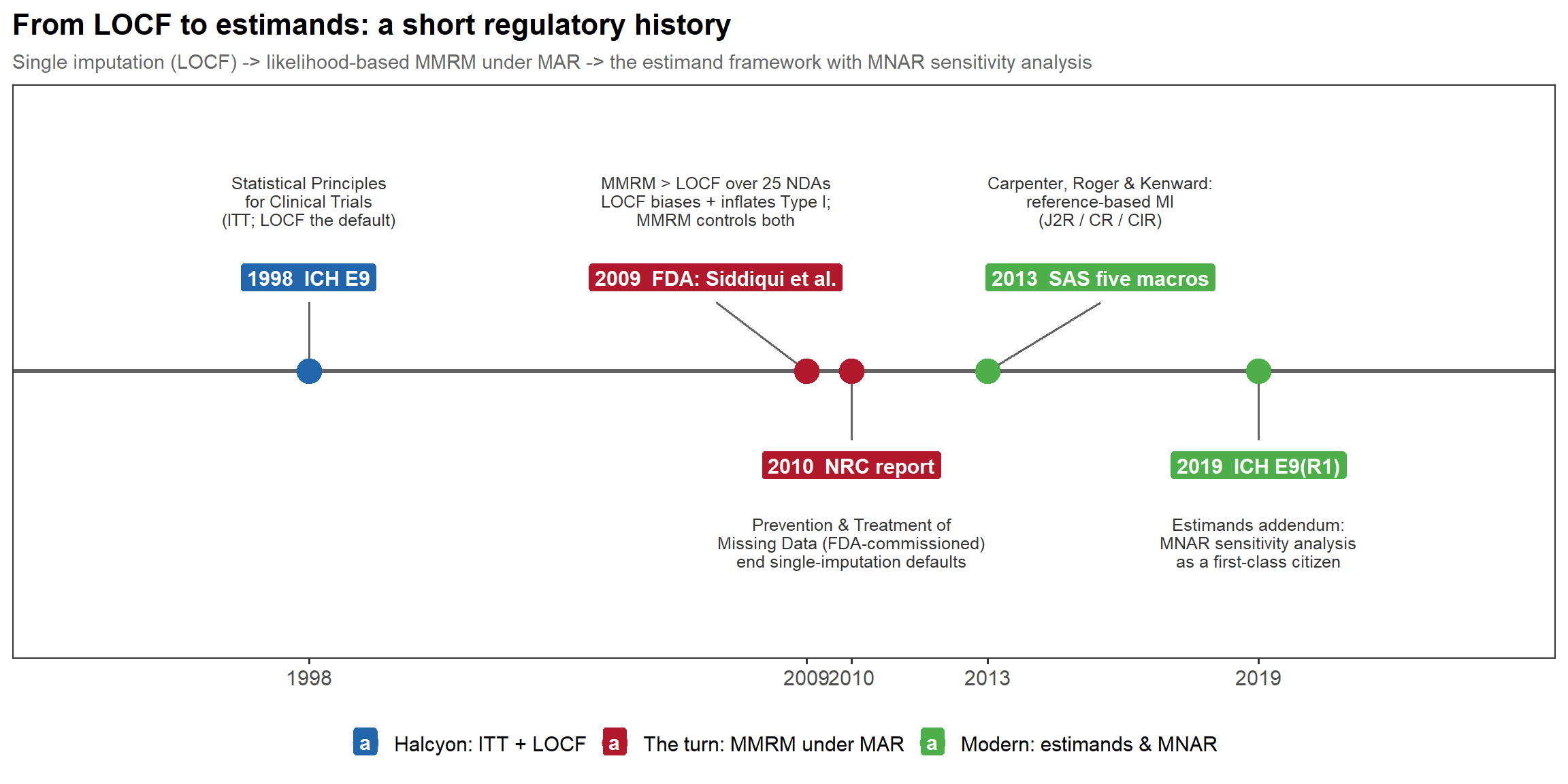
In words: single imputation (LOCF) gave way to likelihood-based MMRM under MAR — pushed by the FDA’s Siddiqui–Hung–O’Neill 2009 review of 25 NDAs and the FDA-commissioned NRC 2010 report — then to the reference-based MI five macros (Carpenter, Roger & Kenward 2013; James Roger / GSK for the DIA working group), and on to the ICH E9(R1) estimand addendum of 2019, which makes MNAR sensitivity analysis a first-class citizen.

1.3 E9 (1998): the bedrock

• The original guideline reached Step 4 on 5 February 1998 and has stood, essentially unchanged, for more than twenty-five years — a remarkable shelf-life for a regulatory document, and a sign of how solid its foundations were.
• It was led and authored-of-record by J. A. Lewis of the UK MCA, who wrote the 1999 Statistics in Medicine note that introduced it to the field.
• Note: it was respected enough that the 2019 update arrived as an addendum bolted onto it, not a revision that swept it away.

1.4 E9(R1) (2019): the addendum

• The addendum had a heavily-consulted gestation — a concept paper in 2014, a draft in 2017, and Step 4 only in November 2019.
• Its central contribution was to standardise the estimand: a disciplined vocabulary of five attributes crossed with five strategies for handling intercurrent events. It systematised an idea that was already latent in E9, rather than inventing a new one from scratch.
• Note: the reception was not uniformly warm — critics called it “old wine in new barrels,” complained that it “ignores causal inference,” and many practitioners found it harder going than its predecessor.

1.5 A caution from Senn

Remember: Stephen Senn grants that the estimand is a basic and useful idea, but he warns against reified marginal or population-weighted estimands — which he calls “misleading and harmful” — and against Lindley’s “confusion between the Greek letter and the reality it represents.” His quarrel is with how the framework is sometimes used, not with the E9(R1) document itself.

1.6 Review of Key Points

• The historical default was single imputation (LOCF); it biases the estimate and under-covers the truth, and that double failure is what set the field in motion.
• The modern frame couples MMRM under MAR with the estimand framework and a serious treatment of MNAR sensitivity analysis.
• The estimand is genuinely useful but contested: the discipline it demands is to name what you are estimating, and then check how much your answer depends on what you cannot see.

Part 2 — Generating the data

2.1 The MADRS depression trial

• Aim: before we can judge any missing-data method honestly, we need a trial whose answer we already know — so we simulate one, and from here on it is the recurring dataset behind every figure in this talk.
• The setting is a two-arm randomised study, active versus placebo, in which each subject is seen at six visits — weeks 0, 2, 4, 6, 8 and 10. The outcome at each visit is the MADRS score — the Montgomery–Åsberg Depression Rating Scale — an integer from 0 to 60, where lower means better.
• In words: the clinician’s question is blunt and singular — does the drug lower the week-10 MADRS more than placebo? — and everything downstream is just an honest attempt to answer it when some patients stop coming.
• Note: because we built the data ourselves, we hold the one thing a real trial never gives us — the true week-10 effect — and we can check, scenario by scenario, whether each method actually recovers it.

2.2 The generating model

• Problem: a single MADRS number is easy to simulate, but a patient gives us six of them, and those six are not independent — a person who starts severe tends to stay severe, and two nearby visits agree more than two far-apart ones. The simulated data has to carry both facts.
• We write each subject’s vector of six values as \(y_i = \mu_i + b_i + E_i\), the sum of three pieces, each with a plain reading.
• The trend: \(\mu_i\) is a per-arm linear time trend — the average MADRS trajectory over the ten weeks, and the only place the treatment effect lives, as a difference in week-10 means between the arms.
• The intercept: \(b_i \sim N(0, \sigma_b^2)\) is a subject random intercept — one scalar, drawn once per patient and added to all six visits alike. In words, patients simply differ in overall severity, and this single number shifts a person’s whole curve up or down.
• The residual: \(E_i \sim \text{MVN}(0, \Sigma_e)\) is an AR(1) within-subject residual, with \(\Sigma_e = \sigma_e^2\, \rho^{|i-j|}\) — the visit-to-visit wobble around a patient’s own curve, whose correlation decays with the separation between visits.

2.3 The generating covariance

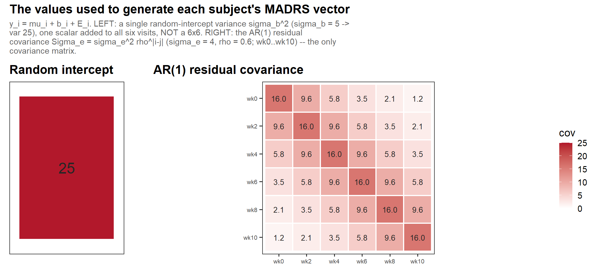
In words: the only covariance matrix in the generation is the AR(1) residual \(\Sigma_e\) (right, \(\sigma_e = 4\), \(\rho = 0.6\)); the random intercept is a single variance \(\sigma_b^2\) (left, \(\sigma_b = 5 \to 25\)) added on top — so the marginal within-subject covariance is simply their sum, \(\sigma_b^2 + \Sigma_e\).

2.4 The treatment effect & the standard scenario

• Aim: to keep the talk legible, we fix one baseline trial and return to it again and again — we call it the standard scenario, and every later experiment perturbs it one knob at a time so we can attribute any change to a single cause.
• The standard scenario is n = 150 per arm, a true week-10 effect of −4 MADRS points (the drug genuinely better), 30% dropout, and crucially no MNAR — the missingness, when we add it, depends only on what we have already observed.
• Note: −4 points is a deliberately modest, realistic signal — large enough to matter clinically, small enough that the variance method and the missingness mechanism can plausibly tip the conclusion. That tension is exactly what the rest of the talk is about.
• Remember: the standard scenario is the anchor, not the whole story — its job is to be the calm baseline against which a single deviation (more dropout, a heavier random intercept, a pinch of MNAR) becomes visible and interpretable.

2.5 Review of Key Points

• Our recurring dataset is a simulated MADRS depression trial — two arms, six visits at weeks 0–10, outcome 0–60 with lower better — and because we built it, we know the truth.
• Each subject’s six values are \(y_i = \mu_i + b_i + E_i\): a per-arm linear trend, a scalar random intercept \(b_i\) added to every visit, and an AR(1) residual \(E_i\) whose correlation decays with visit separation.
• The only covariance matrix in generation is the AR(1) residual \(\Sigma_e\); the random intercept contributes a single variance, and the within-subject covariance is their sum.
• The standard scenario — n = 150/arm, true effect −4 MADRS, 30% dropout, no MNAR — is the baseline we will perturb one knob at a time.

Part 3 — How the data go missing

3.1 Three mechanisms

• Aim: before we can choose an analysis, we have to say how the data went missing — because the honesty of every method downstream rests entirely on which of three worlds we are in.
• MCAR — missing completely at random — is the benign case: a patient is lost for reasons that have nothing to do with their outcome, like a clinic closing or a move out of town. The completers are a fair sample of everyone, and almost any analysis stays unbiased.
• MAR — missing at random — is subtler and far more common: dropout depends only on what we have already seen. A patient whose earlier MADRS visits were poor is more likely to leave, but given those recorded values the missingness carries no extra information. This is the world the MMRM is built for, and where it is valid.
• MNAR — missing not at random — is the dangerous one: dropout depends on the very value that went unmeasured. The patient leaves because this week’s MADRS is about to be bad — a number we never get to record.
• Remember: the distinction is not academic. Under MAR the observed data contain everything we need; under MNAR the reason for leaving is locked inside the measurement we are missing, and no MAR analysis can recover it.

3.2 Diggle–Kenward selection

• Problem: to study MNAR we need a knob that turns it on and off, so that MAR is one end of a dial rather than a different model entirely.
• The Diggle–Kenward selection model gives us exactly that. At each visit a patient’s probability of dropping out is pushed up by their current, about-to-be-missing MADRS through a single parameter γ: the worse the value they are heading toward, the more likely they are to walk out the door before it is recorded.
• Note: the beauty of this construction is the special case. When γ = 0 the current value carries no weight — dropout leans only on the past, recorded visits — and we are back in pure MAR. As γ climbs, missingness starts to feed on the unseen value, and we slide into MNAR. So γ is our MNAR dial, and MAR is simply its zero.

3.2 Diggle–Kenward selection (cont’d)

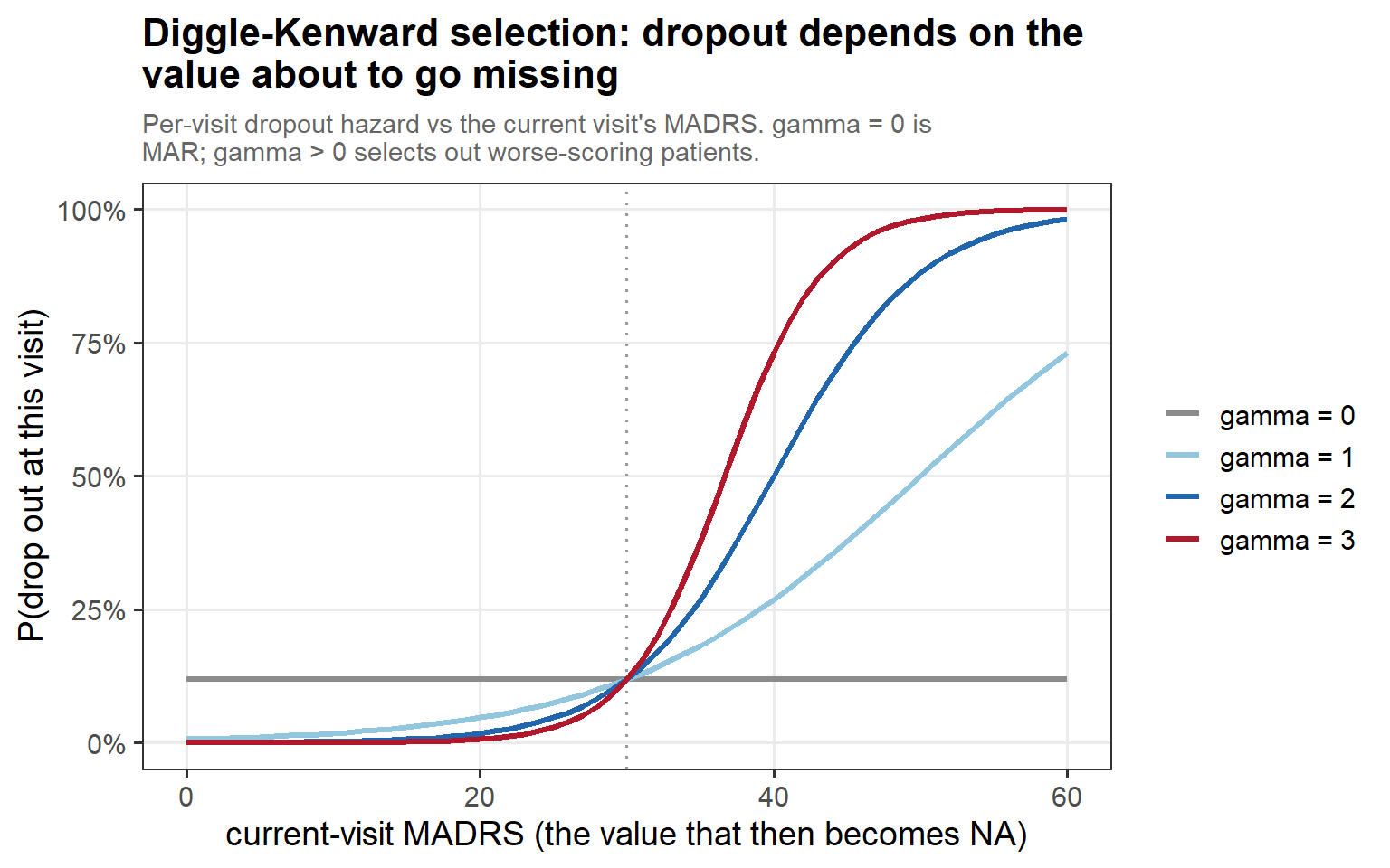
In words: the per-visit dropout hazard rises with the current MADRS, and γ sets the slope — γ = 0 is flat (pure MAR), while γ > 0 selectively pushes out the patients who are about to worsen.

3.2 Selection, in motion

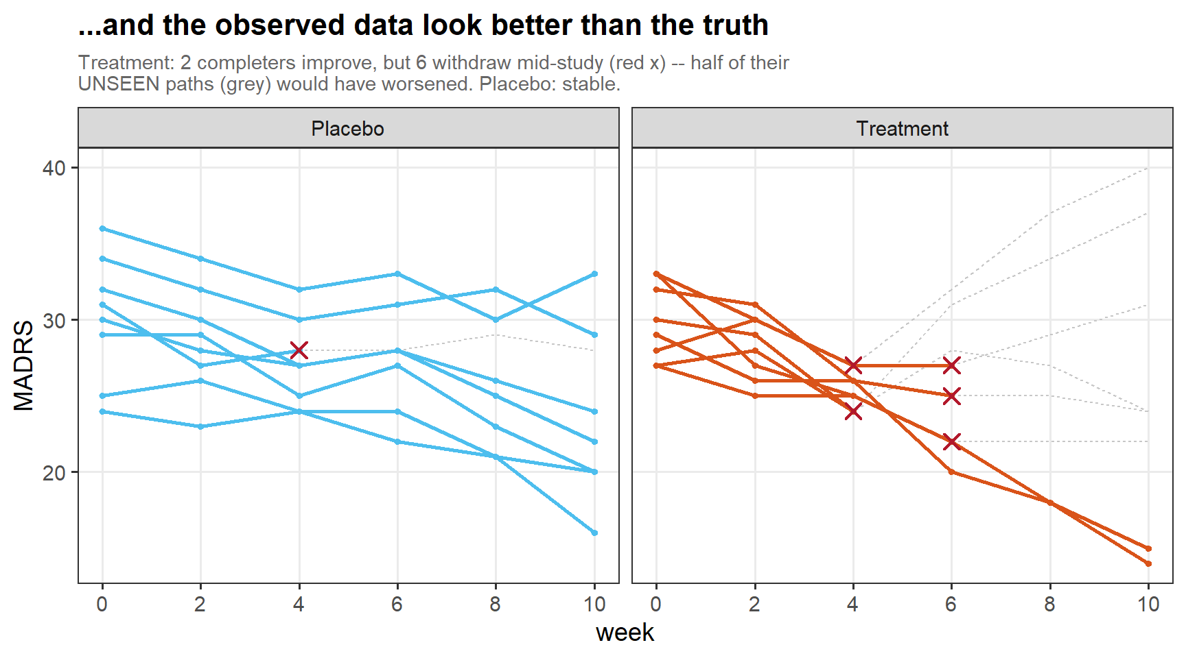
In words: Exaggerated example — the patients who stay are already improving, while those who leave are pulled out exactly as their own paths turn upward. Also their subsequent trajectory is another important but differently parametered story.

3.3 Selection made visible

• Aim: γ is an abstraction until we watch it act on “real” trajectories, so let us follow the patients themselves through the standard depression scenario.
• In words: the patients who stay are the ones doing well — their MADRS trends down, visit by visit. The patients who leave are pulled out precisely as their own paths turn upward, and where those unseen continuations would have gone splits sharply away from the completers.
• However: the analysis only ever sees the completers. With the worsening patients quietly removed, the observed group means drift below the true population means — an optimistic picture that MMRM under MAR has no way of detecting, because every value it can see is perfectly consistent with MAR.

3.4 Two flavours of missingness

• Note: not all dropout has the same shape, and the shape will matter a great deal once we start imputing.
• Monotone dropout is an absorbing tail: once a patient leaves, they are gone for good, so every visit after the exit is missing in one unbroken run. This is the textbook picture, and the one most reference-based methods quietly assume.
• Intermittent missingness is messier and more realistic: a patient skips a single visit — a holiday, an illness, a scheduling clash — and then returns. The gap is an isolated hole punched in the middle of an otherwise complete record.
• Remember: the difference is not cosmetic. Reverting a monotone tail to a reference arm is conceptually clean, but reverting an isolated interior gap forces us to ask exactly which values the reference assumption is meant to touch — and that is the δ-scope distinction that will bite us in Parts 4 and 6.

3.4 Two flavours of missingness (cont’d)

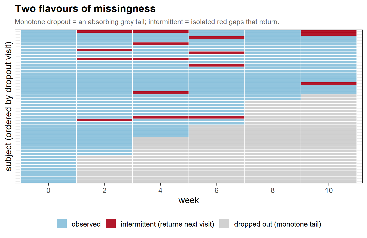
In words: monotone dropout leaves one absorbing tail of missing visits, while intermittent missingness punches isolated gaps into an otherwise complete record — and it is the latter that makes the δ-scope choice consequential.

3.5 Survivor bias

• Problem: suppose the MNAR pressure falls harder on the treatment arm — patients who are about to worsen quietly drop out before that bad visit is recorded, while those still doing well stay on. What does that do to our headline effect?
• The patients who remain on treatment are then a favourable subset: selection has skimmed off some of the worse trajectories, leaving behind a completer group that looks better than the arm as a whole truly is.
• However: the MAR primary analysis takes those survivors at face value. It compares a flattered treatment arm against a more honestly observed placebo arm, and so it overstates the benefit — the drug looks better than it is, purely because of who stayed to be measured.

3.5 Survivor bias (cont’d)

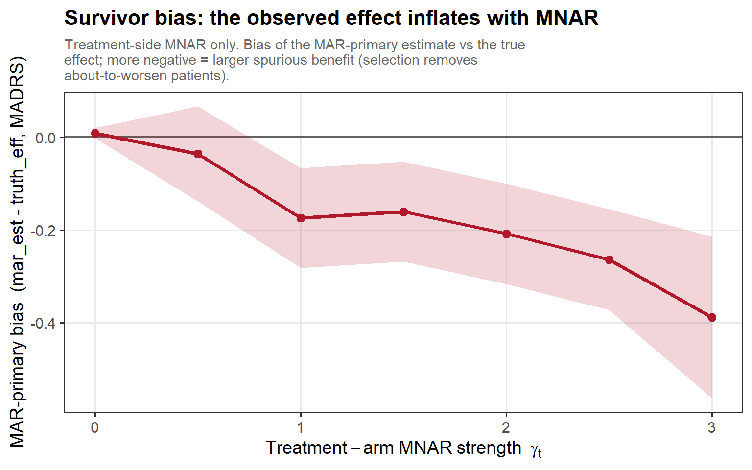
In words: as the treatment-side MNAR strength γ_t grows, the survivors get more favourably selected and the MAR primary overstates the treatment effect ever more — a bias built entirely from who remained.

3.6 Null inflation

• Aim: a test of a primary analysis is the null: when there is no treatment effect at all, how often does the MMRM falsely declare the drug beneficial? That one-sided efficacy error should sit at the nominal 0.025.
• Problem: under MAR, or under MNAR that hits both arms symmetrically, the answer is not reassuring — the efficacy error sits above nominal (~0.06); the excess is a real but not terrible MNAR effect.
• However: the direction of the asymmetry decides everything. Treatment-side MNAR removes the about-to-worsen treated patients, so the completers look better than placebo — a spurious benefit — and the efficacy error climbs to ~0.08, roughly three times nominal. Placebo-side MNAR tilts the other way and fakes a spurious harm — the wrong direction for an efficacy claim, so it does not inflate the error (~0.02).

3.6 Null inflation (cont’d)

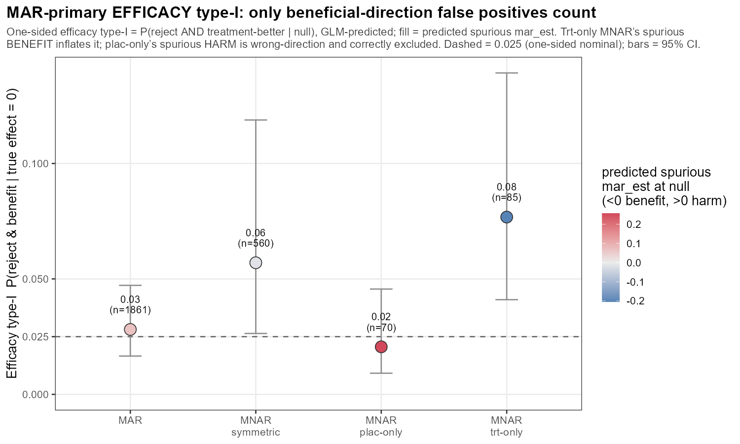
In words: the one-sided efficacy type-I — P(declare benefit | true null), nominal 0.025 (dashed) — holds near nominal under MAR and symmetric MNAR, and is inflated to ~0.08 only by treatment-side MNAR (spurious benefit); placebo-side MNAR makes a spurious harm, the wrong direction, and is correctly not counted.

3.6 Null inflation (cont’d)

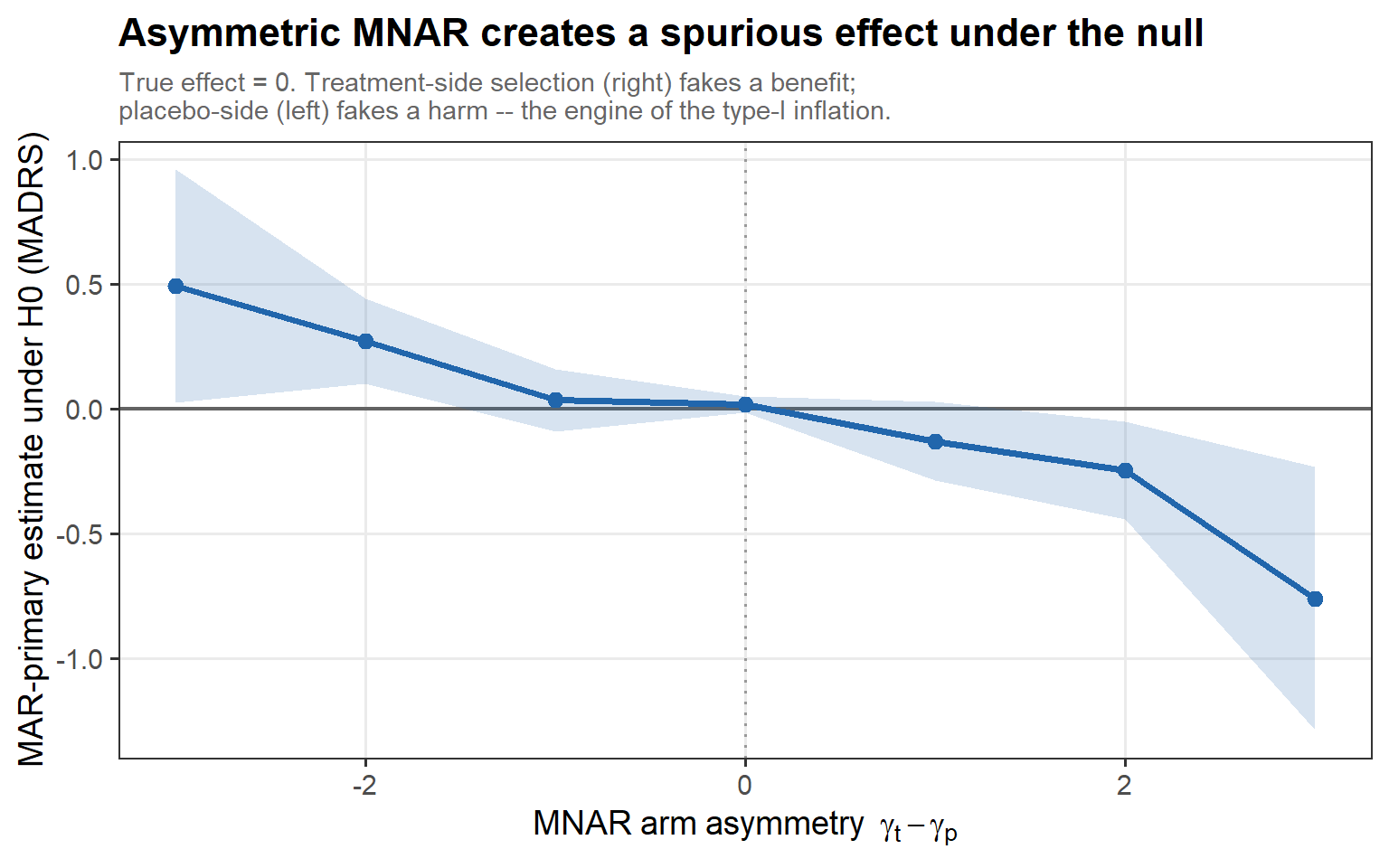
In words: under the true null the estimate drifts with the arm asymmetry γ_t − γ_p — treatment-side MNAR manufactures a spurious benefit, placebo-side a spurious harm. Asymmetric selection conjures an effect out of nothing.

3.7 J2R optimism

• Aim: the standard remedy for MNAR dropout is jump-to-reference (J2R): we assume a patient who leaves the treatment arm loses the benefit and reverts to the placebo reference trajectory. It is traditionally offered as the conservative choice.
• However: look again at who dropped out. Under selection MNAR they did not leave at random — they left because they were worsening. Their true counterfactual path may lie not at the placebo reference but below it; they were perhaps heading somewhere worse than an average placebo patient.
• Note: so J2R is conservative only relative to MAR. Measured against the true, worse-than-reference counterfactual, reverting them merely to placebo could be optimistic — we are imputing a better outcome than the selected dropouts would actually have had.

3.7 J2R is one choice among five

3.7 J2R optimism (cont’d)

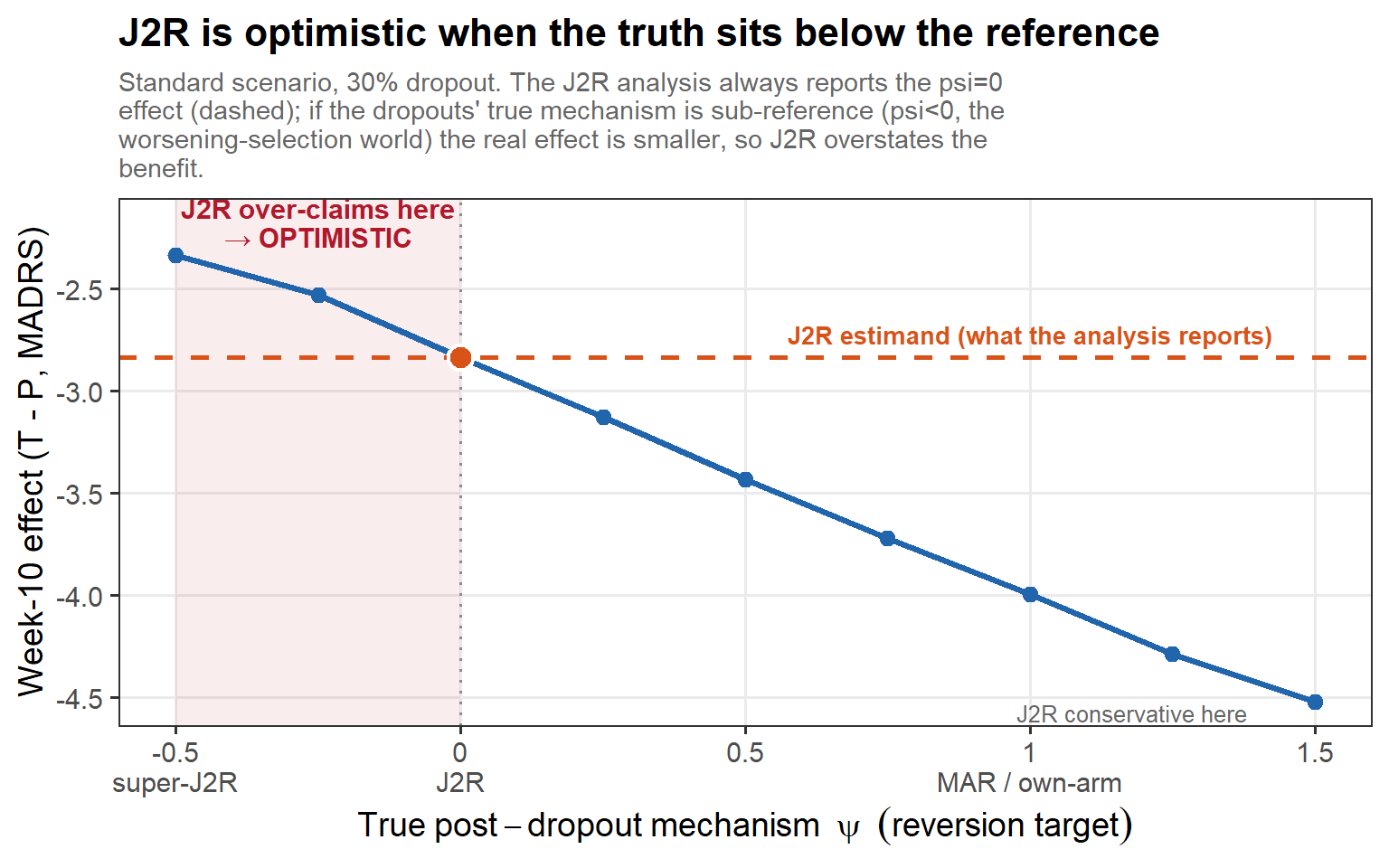
In words: the J2R analysis always reports the reference-reversion effect (the dashed line, ψ = 0). But the true mechanism is whatever nature picks: when selection pulls the dropouts below the reference (ψ < 0, red zone) the real effect is weaker than J2R claims — so J2R is optimistic, not conservative. Only when the truth leans toward own-arm continuation (ψ → 1) is J2R genuinely conservative.

3.7 J2R optimism (cont’d)

Remember: this is why a large tipping point δ at strong MNAR (Part 6) is false reassurance. The tipping procedure bends the imputed values for the missing, but the survivor bias of §3.5 already lives in the observed completers — and no amount of δ on the gaps can reach a bias baked into the data we kept. A reassuring tipping point can sit on top of an analysis that is already wrong.

3.8 Review of Key Points

• Dropout is either MCAR (random), MAR (depends on what we saw), or MNAR (depends on the unseen value); MMRM is valid under MAR, and MNAR is the danger.
• The Diggle–Kenward selection model makes MNAR a dial: γ = 0 is MAR, and γ > 0 selectively drops the about-to-worsen.
• Selection MNAR biases the observed analysis — survivors are a favourable subset, so the MAR primary overstates the treatment benefit.
• Under the null, asymmetric MNAR manufactures a directional effect out of selection: treatment-side dropout fakes a benefit and inflates the one-sided Type 1 error to ( ≈3×{.key} the 0.025 nominal), while placebo-side dropout fakes a harm and does not.
• J2R is conservative only relative to MAR; against the true worse-than-reference counterfactual it may be optimistic, and a large tipping δ is not guaranteed to undo a bias that lives in the survivors.

Part 4 — The reference-based toolkit

4.1 The intercurrent event & the reference idea

• Aim: having committed to MMRM under MAR as the primary analysis, we now ask the question the estimand framework forces on us — what do we believe about a patient after they leave the trial?
• A patient who withdraws early is not simply a hole in the data; the withdrawal is itself an intercurrent event, and the assumption MAR quietly makes is that such a patient would have gone on to improve just as the rest of their own arm did. That “own-arm continues” story credits the dropout with the full treatment benefit they never stayed to receive.
• However: for a drug that works only while it is taken, “own-arm continues” may be far too optimistic, because once the patient stops the treatment the effect plausibly washes out. To note, this makes the estimand a population-level one counting patients who were only partially{.key} treated too(!)
  
• Reference-based imputation answers the post-withdrawal question by borrowing a reference arm — typically placebo — and assuming the withdrawn patient’s trajectory reverts, in whole or in part, toward what an untreated patient would have done.

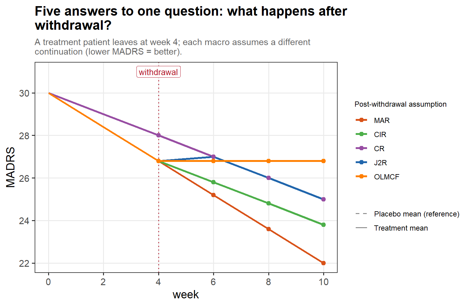
4.2 The five macros

In words: a treatment patient leaves at week 4, and each of the SAS five macros tells a different story about what comes next — MAR keeps following the treatment mean, J2R jumps straight to the placebo (reference) trajectory at withdrawal, CR copies the reference throughout, CIR copies the reference’s increments from the withdrawal value, and OLMCF freezes the last observed value.

4.3 One question, five answers

• Note: the macros are not five competing analyses of the same quantity — they are five different estimands, each encoding a distinct, untestable belief about the unobserved post-withdrawal mean, and the data alone can never tell us which belief is right.
• They form a deliberate ordering of optimism. MAR is the most generous to the experimental arm; J2R — jump to reference — is the conservative default favoured by regulators, because it concedes that the treatment effect vanishes the moment the patient walks out the door.
• The honest way to read this collection is as a sensitivity analysis: not “which macro is correct?” but “how much does my conclusion move as I slide from the optimistic end to the conservative end of this menu?”

4.4 Same data, five estimands

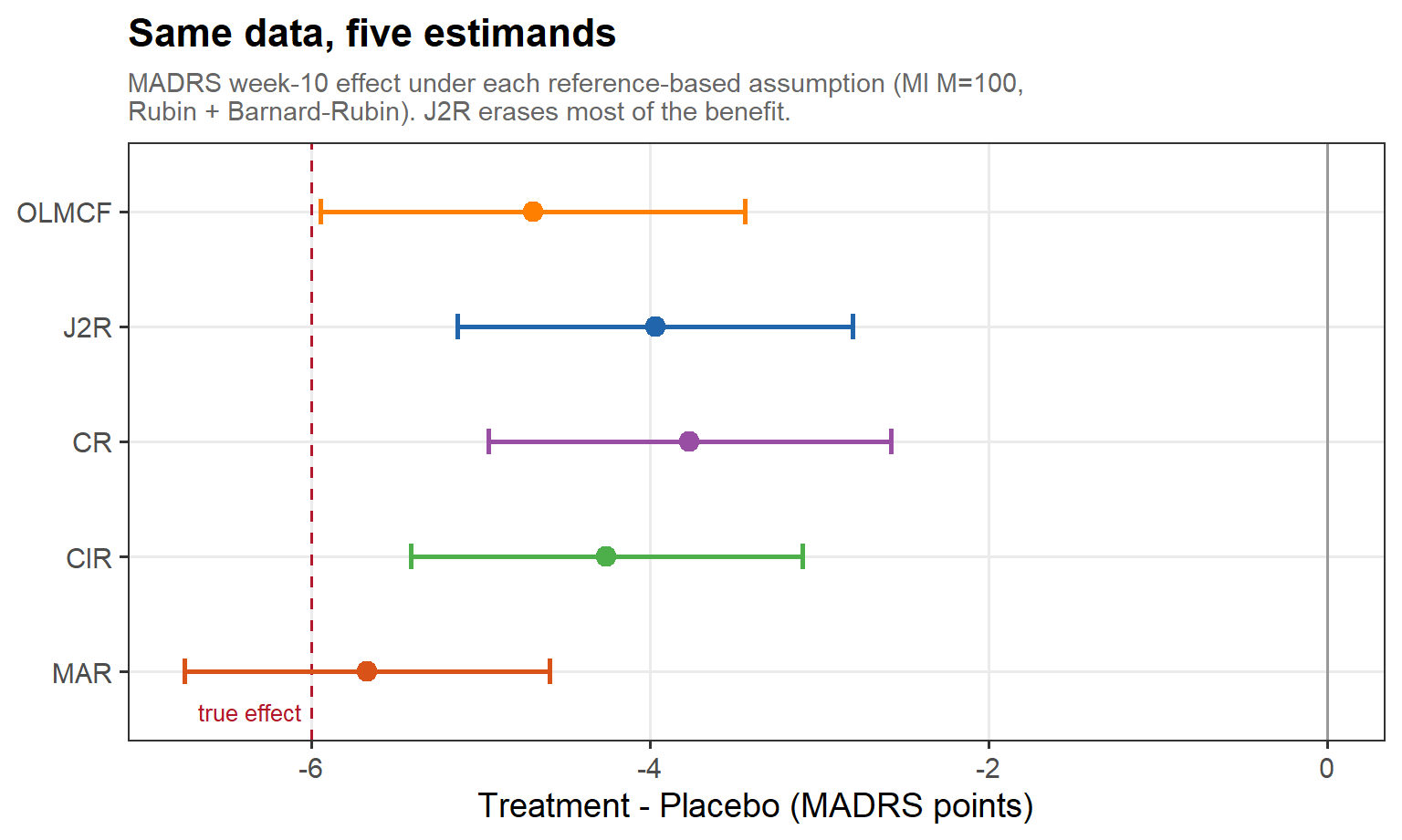
In words: the week-10 treatment effect on one dataset, re-imputed under each assumption (multiple imputation, M = 100, pooled by Rubin + Barnard–Rubin) — MAR recovers essentially the full benefit, while J2R erases most of it; the spread between the points is the sensitivity of the conclusion to an assumption we cannot check.

4.5 The delta convention

• Note: the menu of macros stresses the conclusion by changing the trajectory; a tipping-point analysis stresses it differently, by adding a fixed penalty δ to the imputed values and asking how large δ must grow before significance tips away (we build this out in Part 6).
• Problem: there is a quiet convention buried in where that δ gets added, and the two dominant implementations disagree. rbmi adds δ to every imputed cell, whereas the SAS five macros add it only to the post-ICE (intercurrent event) cells — the visits at or after the intercurrent event.
• Remember: under purely monotone dropout — once a patient is gone, they are gone — every imputed cell is a post-ICE cell, so the two conventions coincide exactly and the discrepancy is invisible.

Example: the moment we admit intermittent missingness — a patient who skips week 6 but returns at week 8 — the two rules diverge, because rbmi penalises that mid-trial gap while the five-macros convention does not. We return to this δ-application gap, and what it does to coverage, in Part 6.

4.6 Review of Key Points

• A withdrawal is an intercurrent event; MAR assumes “own arm continues,” which may flatter a treatment that only works while taken.
• Reference-based imputation borrows a placebo reference; the SAS five macros (MAR, J2R, CR, CIR, OLMCF) span a ladder of optimism, with J2R the conservative default.
• The macros are five estimands, read them as a sensitivity analysis of the conclusion to an untestable assumption.
• The delta convention differs by tool — rbmi adds δ to all imputed cells, the five macros only to post-ICE cells — identical under monotone dropout, divergent once intermittent missingness appears.

Part 5 — Operating characteristics: coverage & variance

The simulation campaign

• Aim: every coverage number in this Part is read off a Monte-Carlo campaign — thousands of simulated trials, each a single design point with a known truth, so that “coverage” is something we can literally count.
• Scale: 23,788 simulated trials to date, costing roughly 176 CPU-days of compute (≈ 4,200 CPU-hours; about 11 minutes per analysis), accumulated by parallel independent workers across multiple devices.
• Per trial: simulate one MADRS trial (~1 sec), add MNAR dropout, fit the MMRM, impute J2R under both δ-scopes, and score nine variance estimators against two estimands (the J2R target and the true effect) — plus the exact tipping δ.
• Design: - mostly - a sparse sampler: each trial perturbs only k ∈ {0, 1, 2} of the knobs away from the standard scenario, the rest held fixed — which is exactly what buys the clean one-knob-at-a-time contrasts the next slides lean on.

Every knob, and its range

The standard scenario sits at the centre; each trial nudges a few of these axes off it:

Axis	Swept range
n per arm	40 – 250
true effect (wk-10 T−P)	−8 → 0 (+ a 10% null at 0)
placebo slope	−0.7 → −0.3 / visit
between-subject SD (σ_b)	3 – 7
residual AR(1) SD (σ_e)	3 – 6
AR(1) correlation (ρ)	0.3 – 0.8
baseline MADRS	28 – 32
dropout fraction	10% – 50%
MNAR strength γ (per arm)	0 – 3, drawn asymmetrically
intermittent-gap probability	0 – 0.15
true mechanism (ψ)	−0.5 → 1.5 (super-J2R → MAR⁺)

Held fixed (for most iterations): unstructured MMRM primary; M (Rubin) = B (bootstrap) = 100; all three proper-MI engines (conjugate / approx-Bayes rbmi / data-augmentation MCMC) run every trial.

5.1 What coverage asks of us

• Aim: we have spent four Parts choosing what to estimate and how to fill the gaps; now we ask the only question that ultimately settles a method — over many repeated trials, does its 95% confidence interval actually contain the truth 95% of the time?
• This single number is coverage, and it is unforgiving in both directions. If the intervals contain the truth less than 95% of the time we have false confidence — we will reject the null too often and declare effects that are not real; if they contain it more than 95% of the time the intervals are needlessly wide, and that wasted width is paid for in lost power.
• Note: coverage is a property of the procedure, not of any one trial — we can only see it by simulating the standard scenario (n = 150 per arm, true effect −4 MADRS, 30% MAR dropout) many times over and counting how often the interval lands on target.

5.1 What coverage asks of us (cont’d)

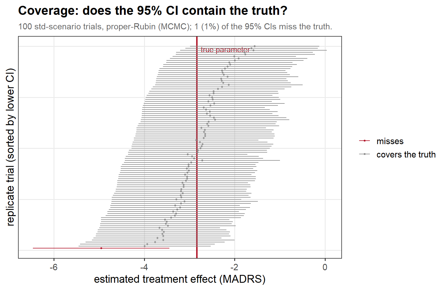
In words: each horizontal bar is one trial’s 95% CI from the standard scenario, sorted by lower bound; the red line is the true parameter, and the red bars that fail to cross it are the misses. A perfectly calibrated 95% interval misses about 1 in 20 — only a percent or two do here, a first hint that the featured method runs slightly conservative.

5.2 The two variance camps

• Problem: once we impute reference-based values, there is no single agreed answer to “how uncertain is the result?” — and the disagreement is a genuine split in philosophy, which will colour everything that follows.
• The first camp is information-anchored: we apply Rubin’s rules to proper Bayesian draws, so that the confidence interval reflects the information a reference-based trial carries — having borrowed the placebo arm to fill the gaps, we deliberately do not claim more certainty than that borrowing earns us.
• The second camp is frequentist-correct: the bootstrap, the jackknife, and the Lu 2014 closed form each try to recover the actual sampling variability of the estimator we computed — the spread we would see if we truly re-ran the trial.
• Remember: these two camps answer different questions, so they will not — and should not — always agree; the rest of this Part is, in large part, a tour of where and why they diverge.

5.2 The two variance camps (cont’d)

Left, red: Frequentist (Bartlett, von Hippel, Lu) Right, blue: Information-anchored (Cro, Carpenter & Kenward)

5.2 The nine methods, honestly

Method	Camp	What it actually is
single	naive	one imputation + the model SE; the over-confident floor
improper	Rubin (improper)	Rubin’s rules on plug-in (point-estimate) imputations
proper_conjugate	info-anchored	Rubin on conjugate (inv-χ² / normal) posterior draws
proper_mcmc	info-anchored	Rubin on data-augmentation Gibbs draws
proper_rbmi	info-anchored	Rubin on rbmi approximate-Bayes draws
boot_v2	frequentist	genuine subject-resampling bootstrap
bootmi	frequentist	bootstrap of MI — double-counts variance †
jack	frequentist	jackknife on conditional-mean imputation
lu2014	frequentist	Lu (2014) closed form, ≈ f² · model-variance

Two confessions: † my bootmi has a bug and double-counts uncertainty — bootstrap-between plus imputation-between variance — so it runs ~1.4× too wide and over-covers; it is not the von Hippel–Bartlett estimator it was first labelled as. And the ugly name boot_v2: the original boot in this corpus was a mislabel (a duplicate of proper-conjugate MI, no resampling at all), so the genuine nonparametric bootstrap had to be re-added as boot_v2.

5.3 Coverage at the standard scenario

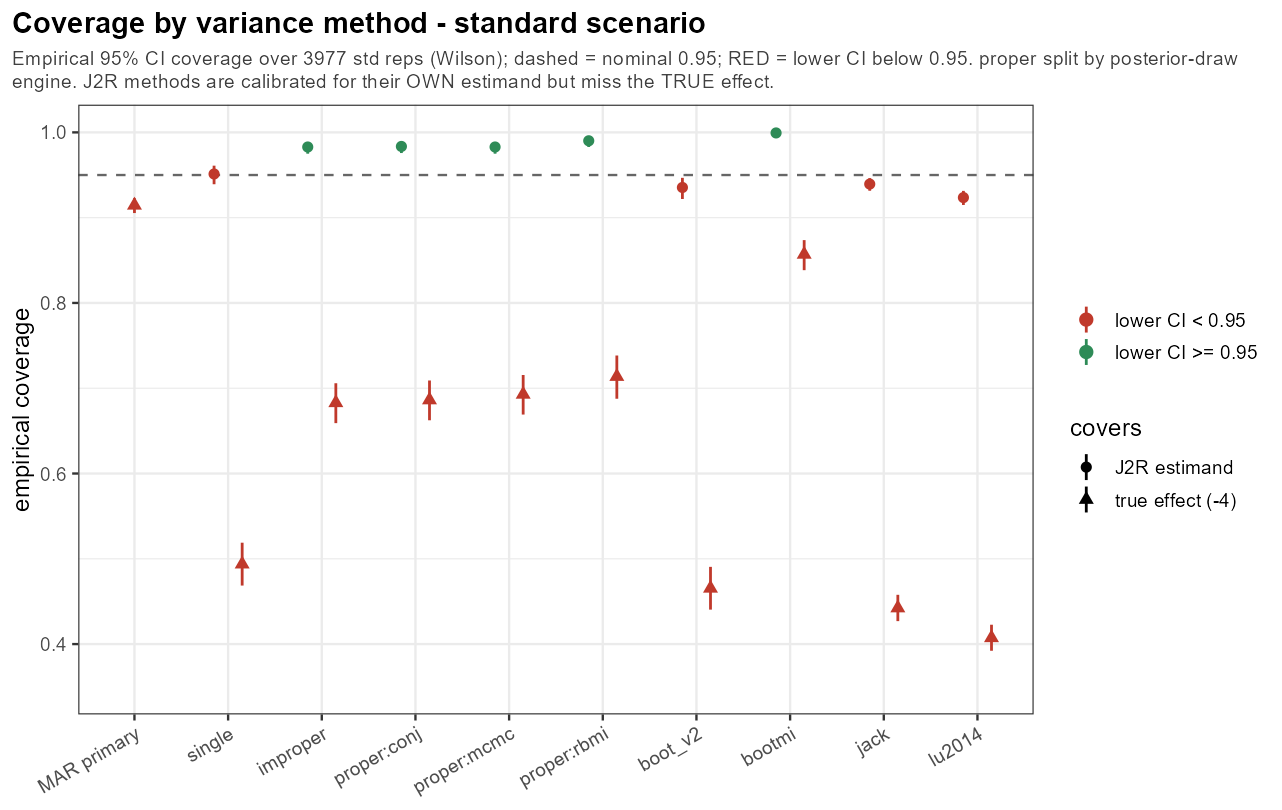
In words: each J2R method covers its own (J2R) estimand far better than the true effect — the information-anchored ones essentially nail it (~0.98), the frequentist ones fall a little short — yet all of them badly miss the true effect; under MAR there is no real dropout-driven shift, so J2R is simply aiming at the wrong target.

5.4 Frequentist variance shrinks with missingness

• Problem: More data tighten the interval around a (purposefully) biased point; a kindred surprise hides in what missingness does to the interval’s width and it is exactly where the two variance camps visibly split.
• The Lu 2014 closed form is, in essence, \(f^2\) times the model variance — and because J2R borrows the placebo arm to fill the gaps, that factor falls as missingness grows: the more we impute from a shared reference, the more certain the closed form believes it has become.
• However: the information-anchored variance does not shrink that way — it keeps faith with how little a borrowed arm truly tells us — and the gap between the two widths, opening up exactly as dropout rises, is the mechanical source of the over-coverage that decides the method comparison.

5.4 Frequentist variance shrinks with missingness (cont’d)

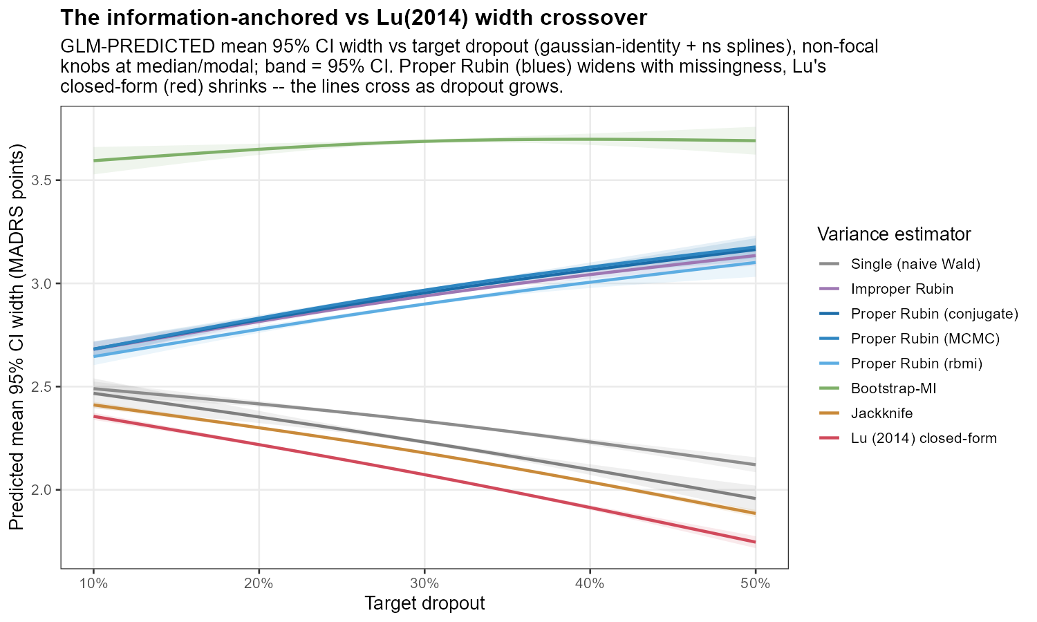
In words: as the missing fraction grows the frequentist (Lu-style) width bends downward while the information-anchored width holds; the two curves cross, and the widening gap to their right is precisely the over-coverage we reach in §5.9.

5.5 One knob at a time

• Aim: the data-generating spine has roughly a dozen knobs — sample size, effect size, baseline severity, the variance components, the dropout rate, the MNAR strength — and turning them all at once would be very hard to interpret.
• So we instead hold the standard scenario fixed and turn one knob at a time, asking of each: does it leave coverage alone, or does it bend it? We walk through every knob on the slides that follow — each is one column of the pass/fail scorecard we assemble in §5.9.
• Note: A fuller sweep with modelling concurrent changes with a GLM bolted onto the results are in the works.

5.6 One knob: asymmetric MNAR

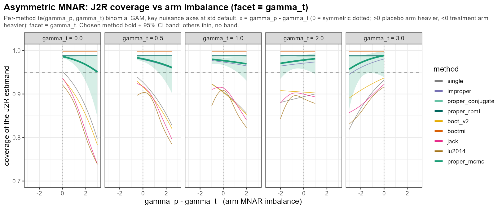
In words: when the two arms drop out for different reasons — asymmetric MNAR — the frequentist intervals degrade the hardest, while the information-anchored ones largely hold; this arm imbalance is the sweep’s sharpest stressor for the frequentist camp. (Note: this is a misnomer, we are turning two knobs at a time.)

5.6 One knob: the true mechanism

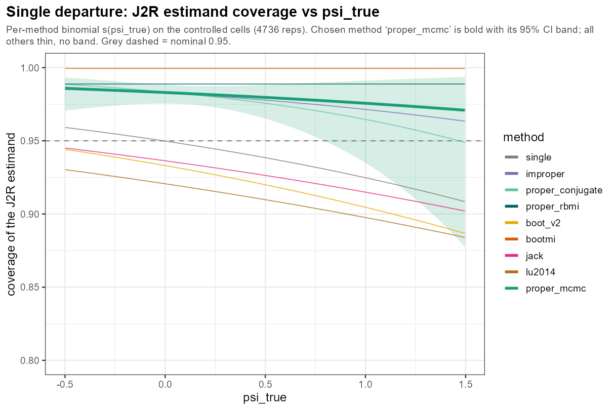
In words: sliding the true post-dropout mechanism away from J2R steadily erodes coverage — the method is calibrated only at the assumption it was built on, and pays for every step nature takes away from it.

5.6 One knob: sample size

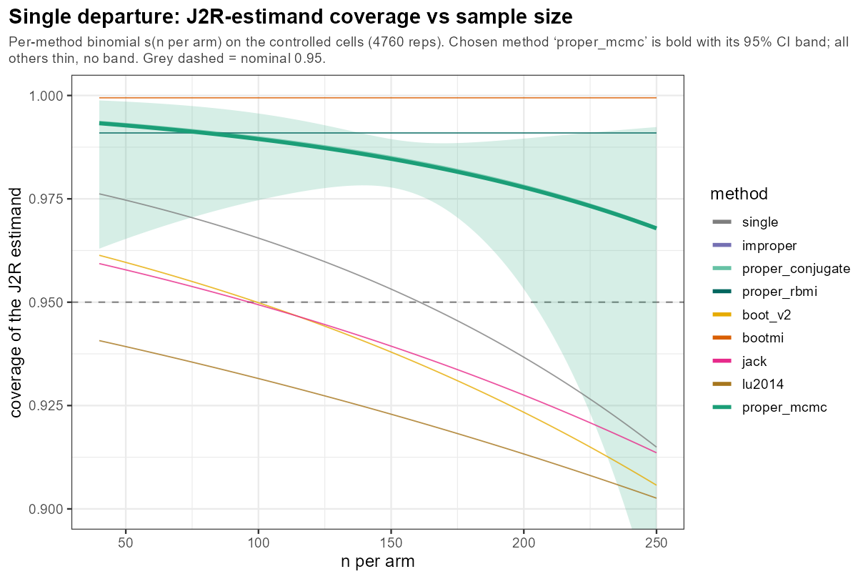
In words: as n per arm grows the J2R-estimand coverage holds its line near 95%, while true-effect coverage drifts downward — a larger trial buys precision around the J2R target, not around the effect a clinician cares about.

5.6 One knob: true effect

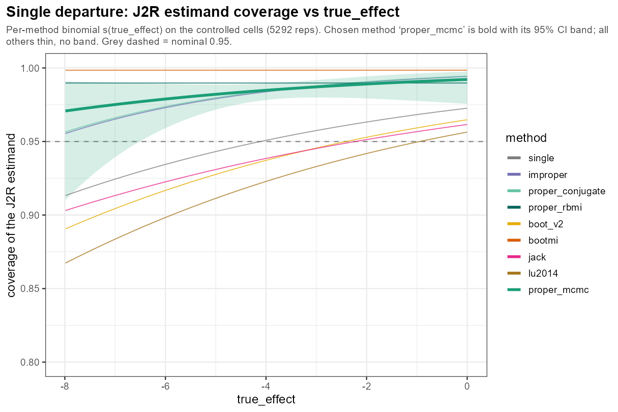
In words: sweeping the true week-10 effect from null to −8 leaves the coverage pattern unmoved — information-anchored methods near/above 0.95, frequentist a little short — so effect size alone is not a coverage stressor.

5.6 One knob: baseline severity

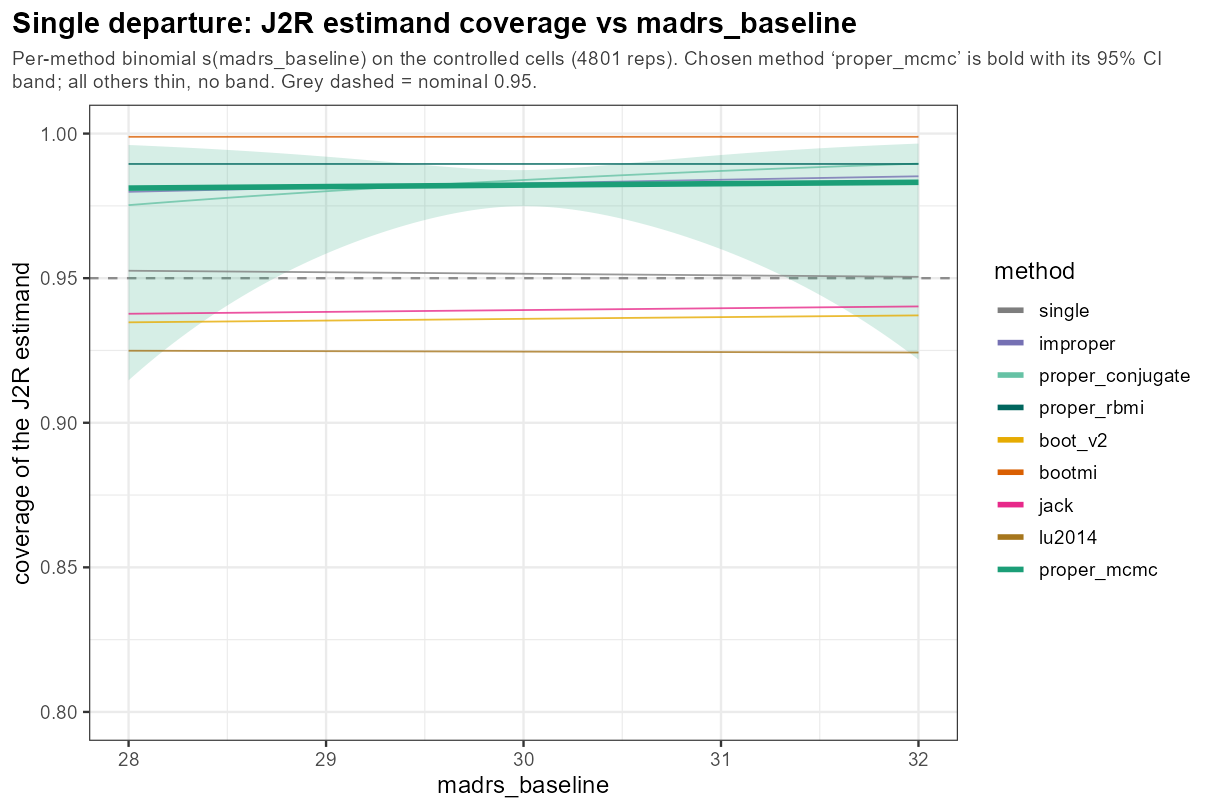
In words: baseline MADRS across its clinically plausible 28–32 band leaves coverage flat — a benign knob, with every method holding its place.

5.6 One knob: placebo slope

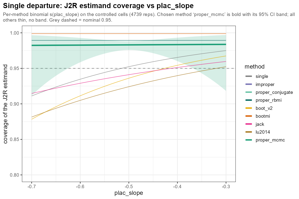
In words: the placebo-arm slope — how fast the reference itself improves — barely moves coverage; the method ordering is unchanged across its range.

5.6 One knob: between-subject SD

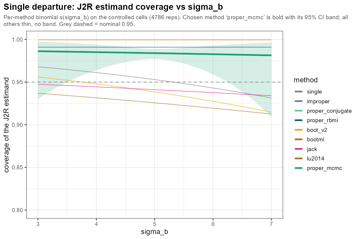
In words: the between-subject SD σ_b (how widely patients differ in overall severity) leaves coverage essentially flat — benign.

5.6 One knob: residual SD

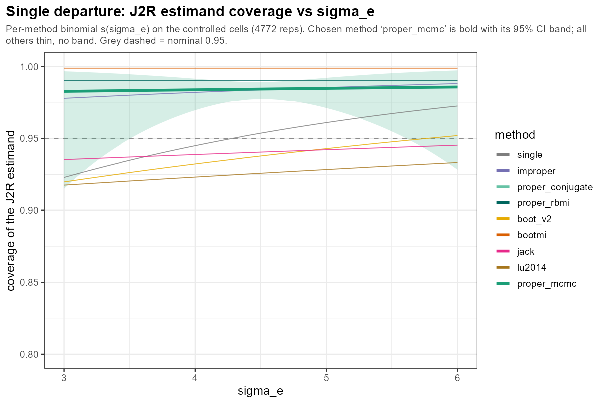
In words: the residual SD σ_e (visit-to-visit noise around a patient’s own curve) leaves coverage essentially flat — benign.

5.6 One knob: AR(1) correlation

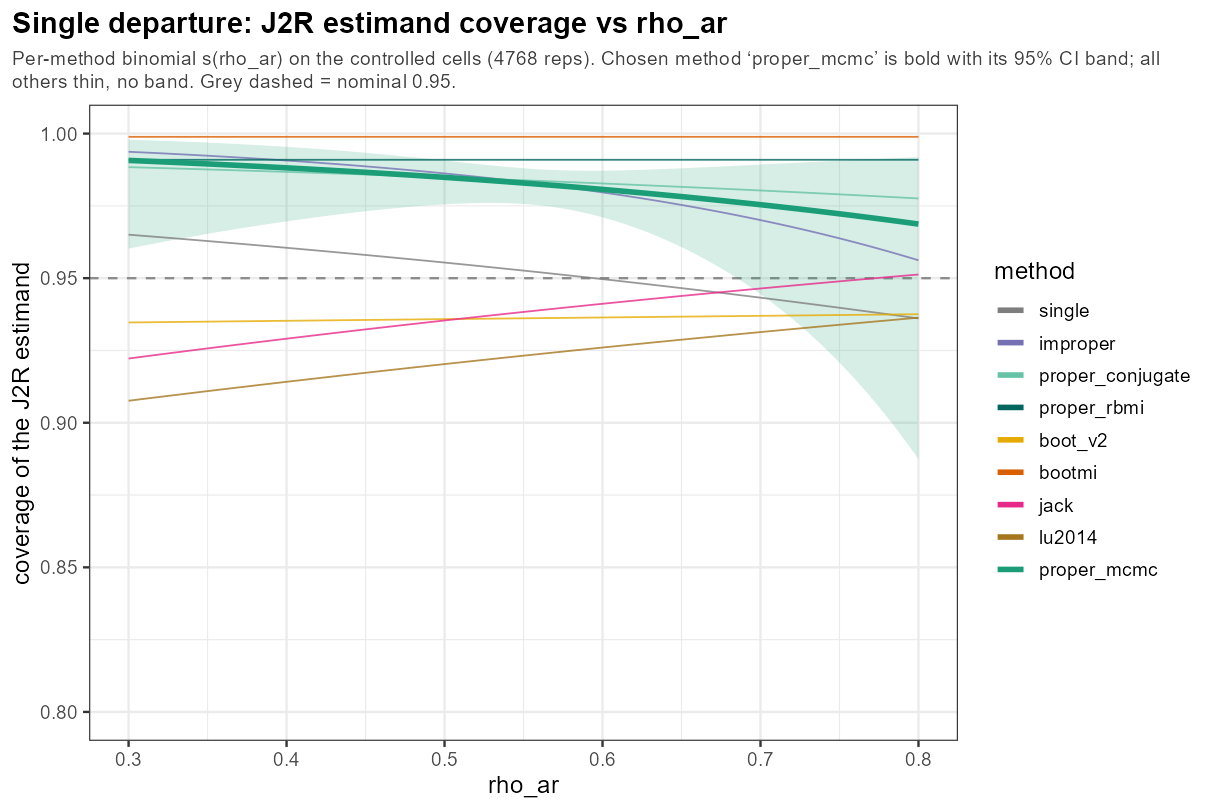
In words: the AR(1) correlation ρ — how much nearby visits agree — barely bends coverage across 0.3–0.8; another benign knob.

5.6 One knob: dropout rate

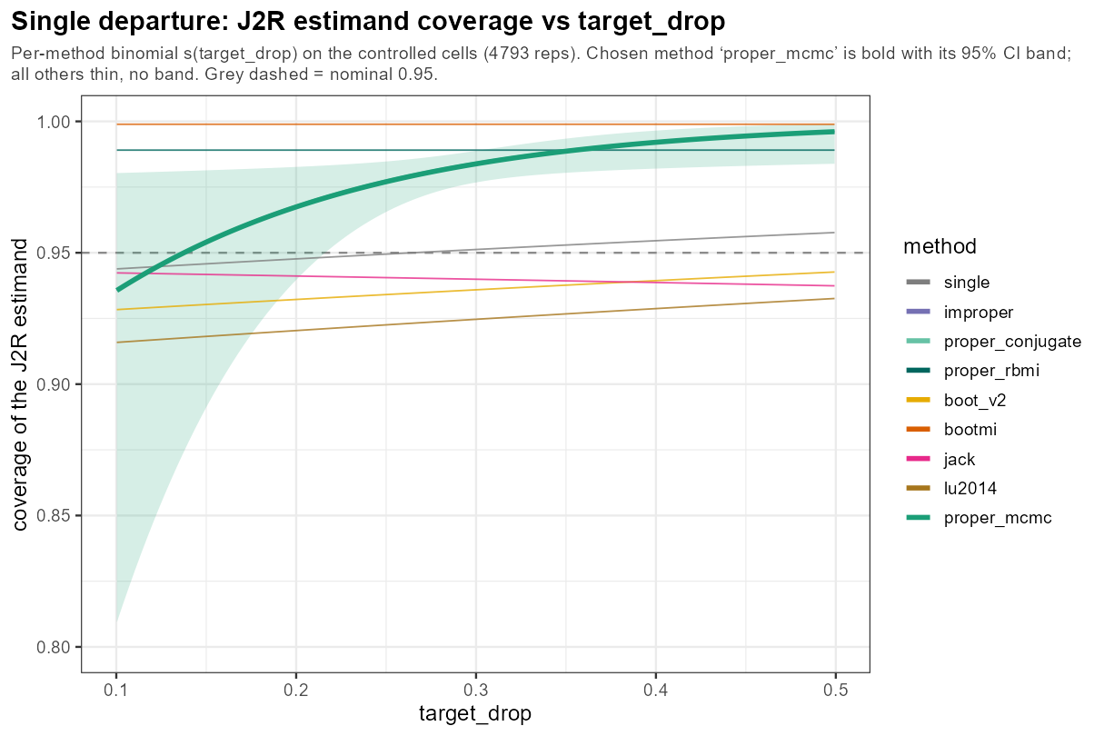
In words: the dropout rate is the one knob where even the information-anchored methods slip below 0.95 — at low dropout, when little is imputed, the J2R estimand is hardest to cover and the proper methods dip to ~0.94, climbing to over-coverage as dropout grows; the frequentist intervals sit lower still throughout.

5.6 One knob: intermittent missingness

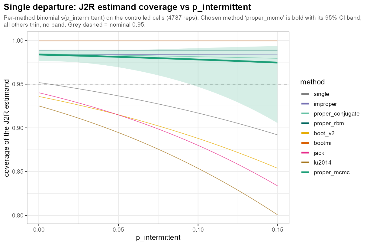
In words: intermittent missingness — isolated interior gaps rather than a clean tail — erodes the frequentist methods the most (toward ~0.85), the δ-scope-sensitive knob, while the proper methods hold.

5.7 The regret matrix

• Aim: we can now assemble the whole story into a single picture — we pick a variance method and nature picks the true post-dropout mechanism, and we score the outcome by the coverage of the per-mechanism estimand, the target that is actually correct for whatever nature chose.
• The hope, going in, is to find one row — one method — that stays calibrated no matter which column nature plays; that row would be the method we recommend without caveat.
• Note: the matrix below is read like a heat map — white cells are calibrated near 0.95, red cells under-cover, blue cells over-cover — and the punchline is in what we will not find.

5.8 The regret matrix (cont’d)

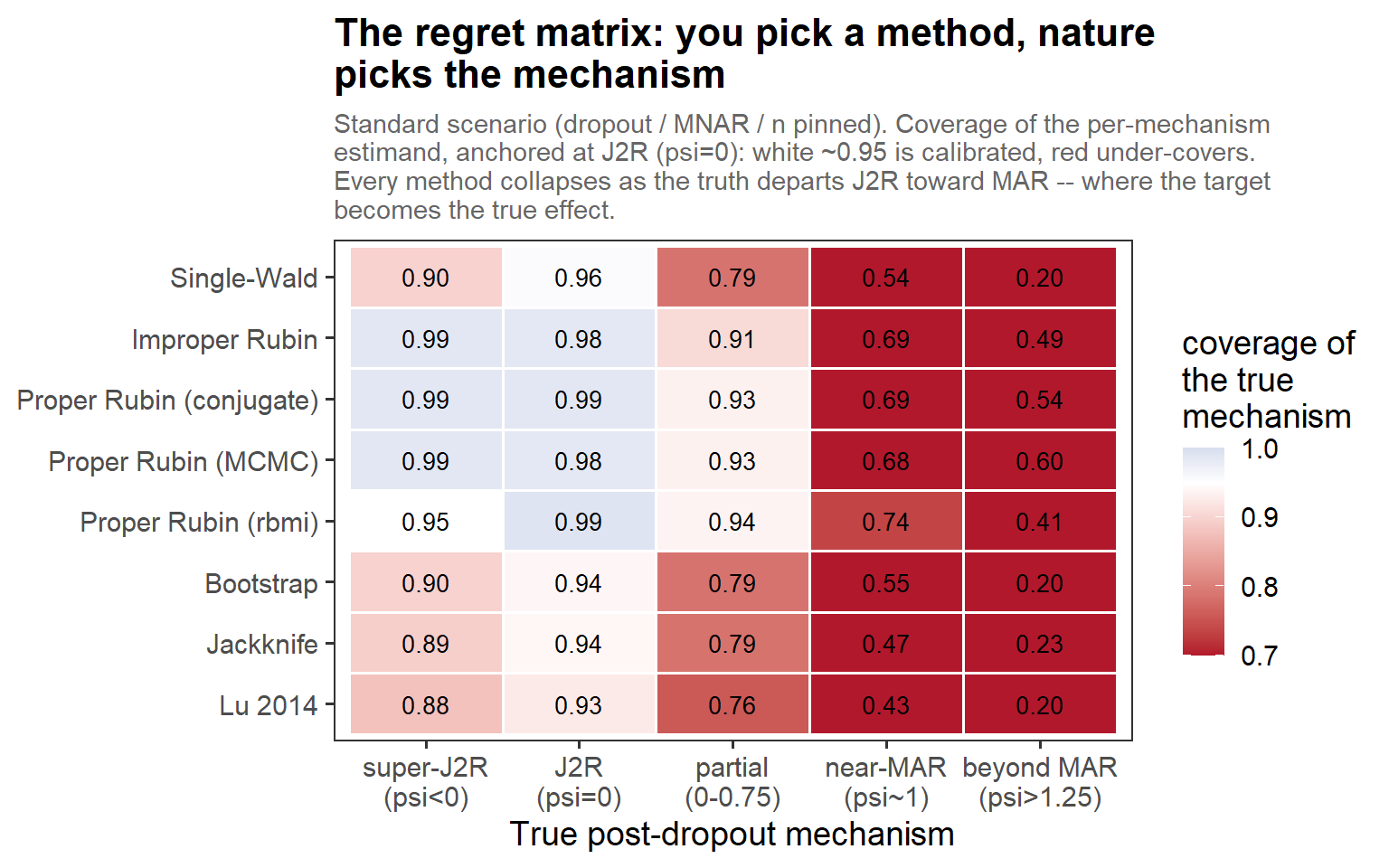
In words: nuisances pinned at the standard scenario, so each column is a clean cut of the true mechanism. There are calibrated islands at the J2R column (ψ = 0) — the three proper engines agree — but every method collapses as the truth departs toward MAR, where the per-mechanism target is the true effect. No row is blur everywhere.

5.8 At the J2R estimand, under stress

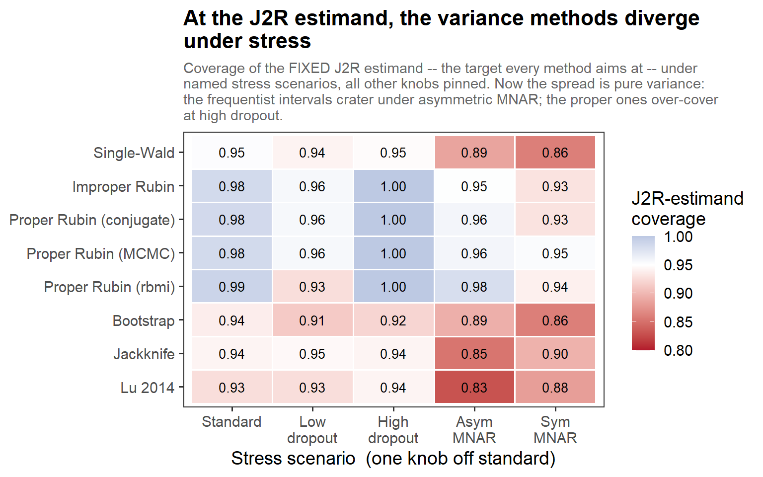
In words: the matrix above fixed the target (ψ); here we move the stressor instead, so the spread is pure variance. The frequentist intervals (bootstrap, jackknife, Lu) crater under asymmetric MNAR (~0.83–0.89), while the information-anchored proper engines hold (~0.96–0.98); at high dropout the proper ones tip into over-coverage (1.00). Same nine methods, two failure modes — bias on the left matrix, variance on this one.

5.9 The highest coverage is not the best method

• Problem: it is tempting to crown the method with the highest coverage — the one whose intervals almost never miss but that instinct may not be optimal, because an interval can hit the truth simply by being too wide to miss anything.
• The buggy bootstrap-MI method (bootmi) passes every single knob in the sweep — its coverage sits at essentially 1.00 everywhere — so on the pass/fail scorecard it looks “flawless”, and a quick reading would name it the champion.
• However: it earns that perfect score only by being roughly 1.4× the MAR-primary width — its near-perfect coverage is over-coverage, and the safety it appears to buy is paid for in lost power, the very cost Section 5.1 warned us about.

5.9 The highest coverage is not the best method (cont’d)

5.9 Coverage vs width

• In words: The scatterplot is the whole argument. bootmi sits top-right — highest coverage, but the widest interval — buying its coverage with width.
• Coverage rises smoothly with width down the rest of the field: the information-anchored proper-Rubin methods reach ~0.98 at moderate width, while the frequentist methods (bootstrap, jackknife, Lu) are the narrowest but dip below 0.95.
• Remember: there is no free lunch on this curve — width buys coverage. The honest question is never “who covers most?” but “who reaches ~0.95 at the smallest width?” Over-coverage is just lost power wearing a clean scorecard.

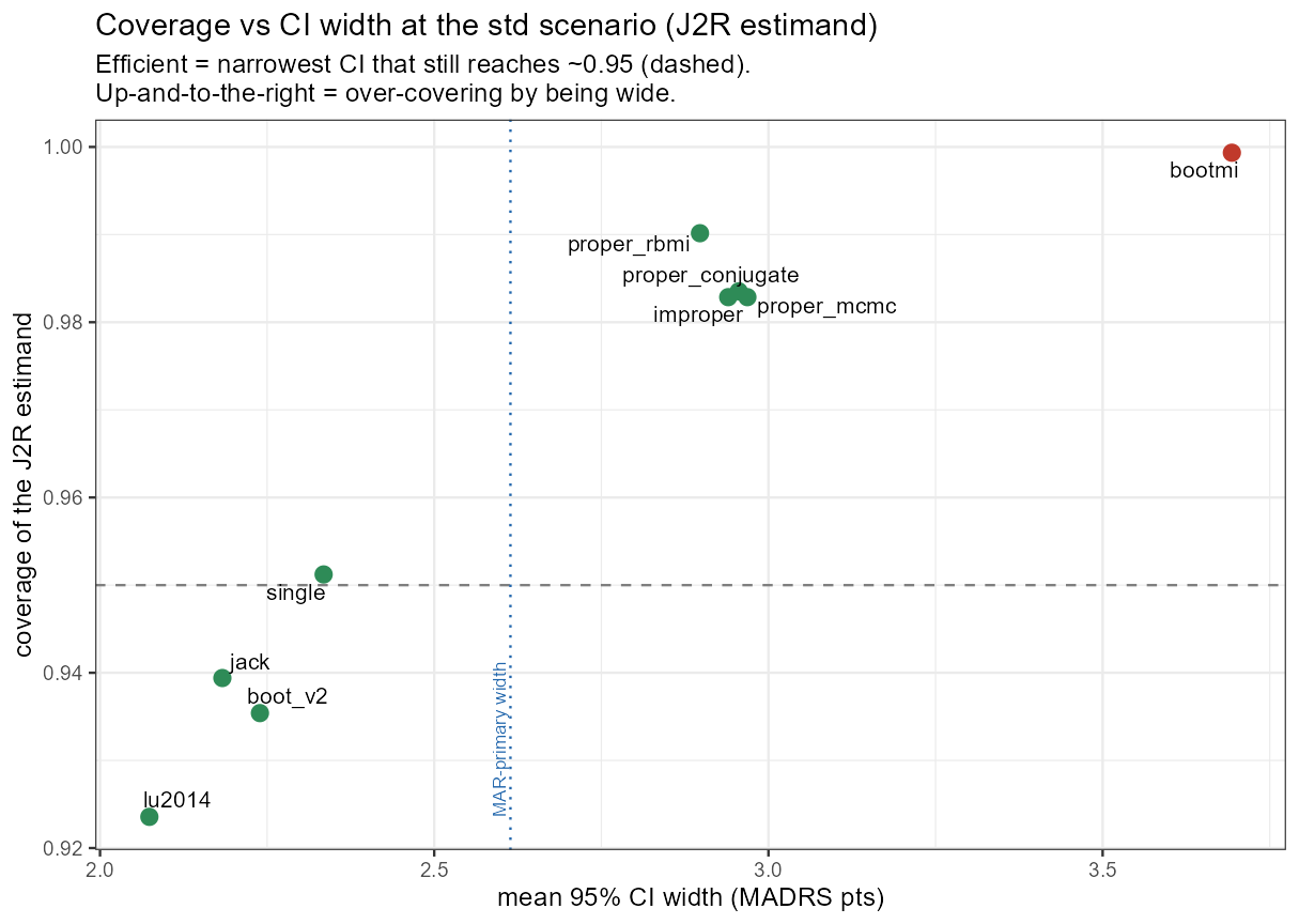
5.9 The highest coverage is not the best method (cont’d)

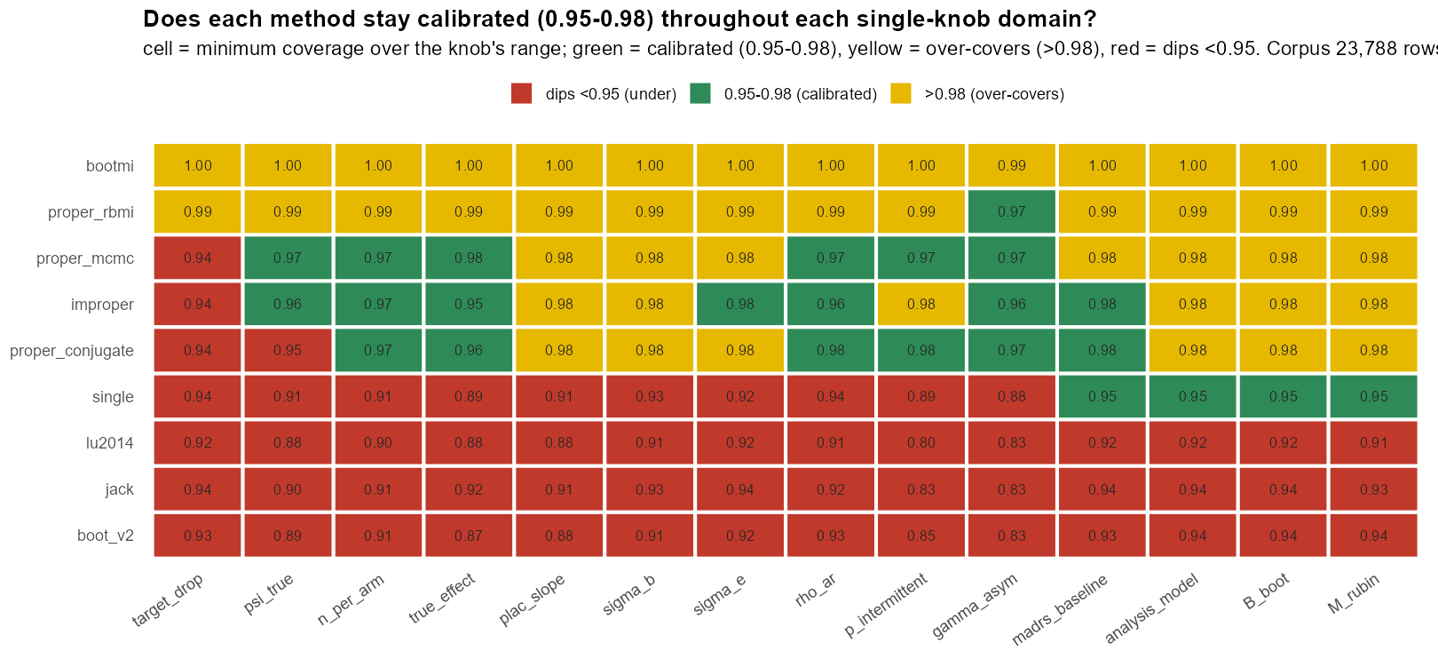
In words: the scorecard reads in three colours — red = dips below 0.95, green = the calibrated 0.95–0.98 band, yellow = over-covers (>0.98). bootmi is yellow everywhere — it passes only by over-covering; the proper-Rubin rows are mostly yellow (slipping red only at the dropout extremes); the frequentist rows are red. “Passing” this scorecard mostly means over-covering, not being calibrated.

5.9 The verdict

• bootmi’s flawless scorecard is a variance double-counting artefact — it stacks bootstrap-between on top of imputation-between variation (~1.4× the MAR-primary width) — not principled conservatism.
• The frequentist intervals (bootstrap, jackknife, Lu 2014) are narrow but under-cover the J2R estimand (~0.92–0.94), sitting below the MAR-primary width.
• The calibrated pick is the information-anchored proper-Rubin interval — featured throughout as proper_mcmc (Rubin’s rules on data-augmentation MCMC draws). It is the most uniformly calibrated of the proper family: ~0.98 at ~1.14× the MAR-primary width, holding across every knob but one — the dropout extreme, where it dips only to ~0.94.

5.10 Review of Key Points

• Coverage is the one verdict that matters: a 95% CI should contain the truth 95% of the time — no fewer (false confidence) and no more (wasted width, lost power).
• The two camps answer different questions: information-anchored variance (Rubin on proper draws) reflects the information a borrowed-arm trial really has, while frequentist-correct variance (bootstrap, jackknife, Lu 2014) chases the estimator’s sampling spread — and they part ways as missingness grows.
• Every J2R method covers its own estimand far better than the true effect under MAR (the information-anchored ones essentially nail it, the frequentist ones fall a little short).
• The regret matrix has no row that is grrat everywhere: methods are calibrated only near the assumption they were built on. Asymmetric MNAR craters the frequentist intervals while the proper ones absorb it to a degree; the one place even the proper methods slip below 0.95 is the extremes of dropout.
• The highest coverage is not the best method — bootmi aces every knob only by being ~1.4× too wide, and the narrow frequentist intervals under-cover; the calibrated pick is the information-anchored proper-Rubin interval (proper_mcmc, ~0.98 at ~1.14× the MAR-primary width, the most uniformly calibrated of the proper family).

Part 6 — The tipping point

6.1 The tipping-point procedure

• Problem: we have leaned on jump-to-reference (J2R) as our conservative default, but even J2R is a choice — it assumes the people who left lose exactly the active-arm benefit and no more, and a sceptical reviewer may suspect they did even worse than that.
• Aim: rather than defend one assumption, we ask how far we would have to bend it before the conclusion gives way. The tipping-point procedure does this mechanically: we add δ MADRS-points to the imputed values, re-fit the model, and raise δ — making the unseen patients steadily worse — until the treatment effect loses significance.
• In words: the tipping δ is the smallest penalty that overturns the result. If that δ exceeds any clinically plausible shift, then no believable departure from MAR can erase the finding, and we declare it robust to MNAR.

6.2 The δ-sweep

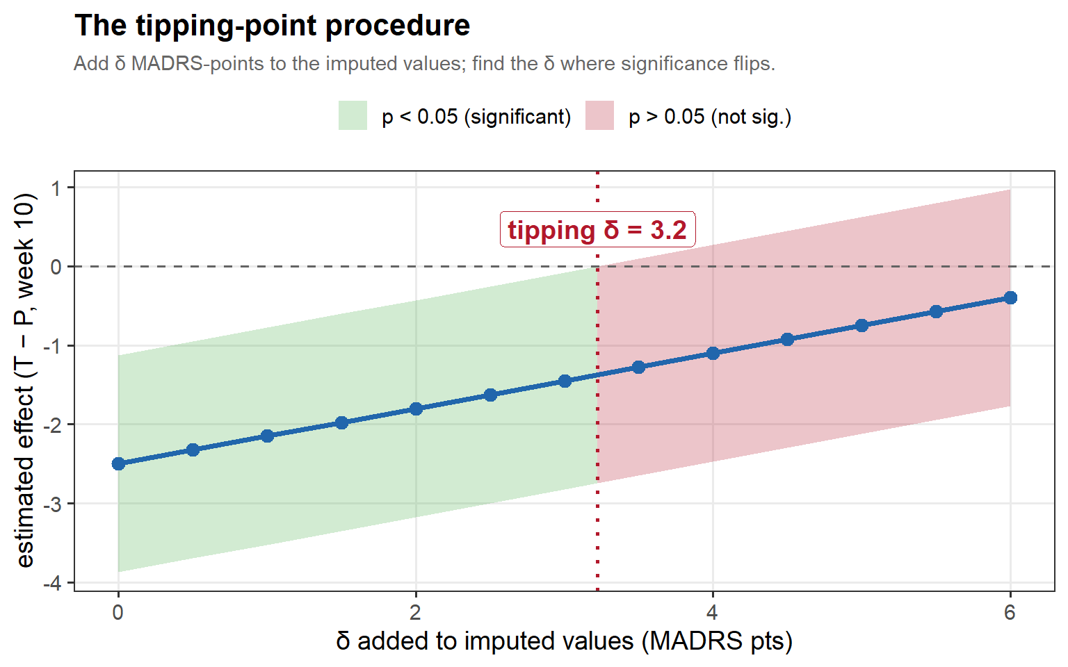
In words: as we add δ, the estimate is dragged toward the null and the confidence band climbs through zero; the tipping δ (red) is the first point at which the interval can no longer exclude no-effect. The wider the cushion before that line, the more robust the result.

6.3 Where δ is applied: rbmi vs SAS

• Note: the procedure hides a subtlety that can move a borderline submission — which imputed cells the δ actually touches. The two mainstream implementations answer this differently.
• In words: rbmi adds δ to every imputed value for a withdrawer, whereas the SAS five-macros add it only to the post-ICE cells — the visits strictly after the intercurrent event. Under clean monotone dropout, where everything after withdrawal is missing, the two are identical; they diverge precisely when intermittent missingness sprinkles gaps before the dropout.
• Remember: this is not a bug in either tool but a genuine convention gap, and a δ that looks robust under one scope can be made to tip earlier under the other.

6.4 The two δ-scopes, drawn

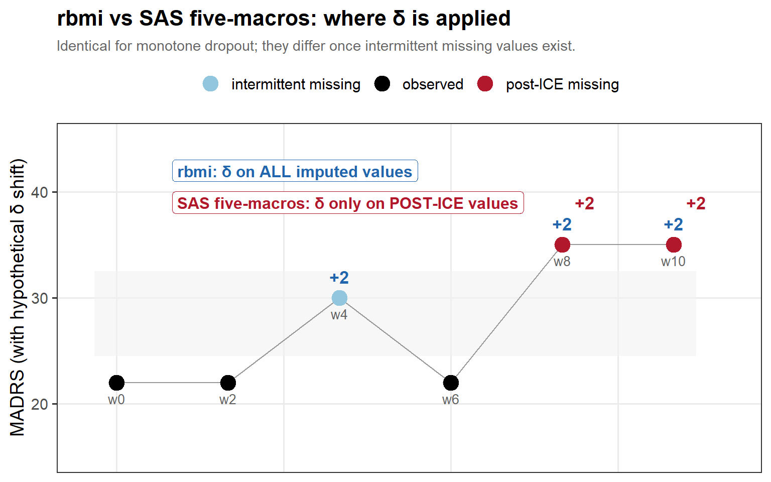
In words: for this patient, both conventions penalise the post-ICE visits (red, +δ), but only rbmi also penalises the earlier intermittent gap (the grey band) — so under intermittent missingness rbmi applies the heavier total shift and tips sooner.

6.5 The tipping point at the standard design

• Aim: before we vary anything, it is worth pinning the procedure to our recurring anchor — the standard scenario of n = 150 per arm, a true effect of −4 MADRS, and 30% MAR dropout — and asking what a single, fixed design buys us.
• In words: one might hope that a fixed scenario yields a single robustness margin, but it does not: across replicate trials the tipping δ has a genuine spread, because each trial’s sampling noise shifts how close the primary result already sits to the null.
• Remember: the tipping δ is therefore an estimate, not a constant — and like any estimate it deserves to be read as a distribution rather than a single reassuring number.

6.6 A distribution of robustness margins

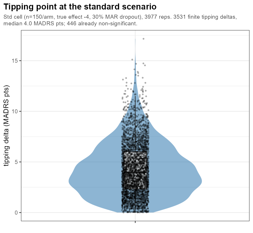
In words: even at one frozen design the tipping δ fans out across trials; the bulk sits comfortably above any plausible 2-point shift, but the lower tail is a reminder that some trials are far more fragile to MNAR than the headline average suggests.

6.7 Does the tipping δ know the truth?

• Problem: the tipping δ is meant to be a barometer of robustness, so we should ask the honest question — does it actually track how much MNAR is really present, or is it blind to the very thing it is supposed to guard against?
• However: Across the whole randomized corpus, the tipping δ looks almost flat in the true MNAR strength — which is understandable since MNAR strength cannot be inferred from the data.
• Note: that marginal flatness is a confounded view. Once we hold the rest of the design fixed and sweep a single axis — letting only the active-arm MNAR slope γ_t move — a clean response appears, unfortunately in the opposite direction.

6.8 The MNAR-connection

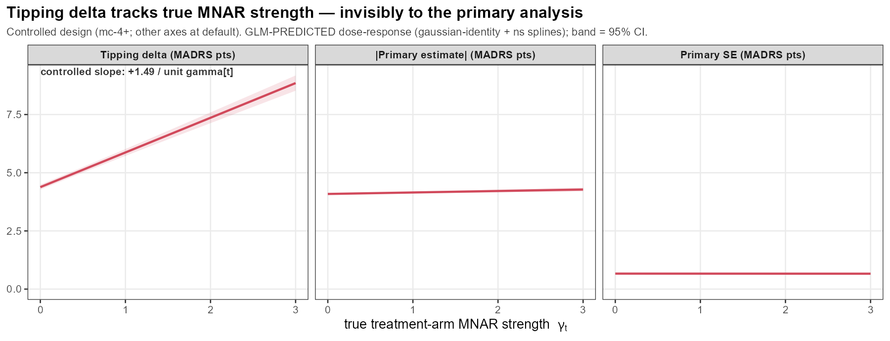
In words: as the true active-arm MNAR slope γ_t grows, the tipping δ rises]{.key}! This means that when a worrysome feature exist in the study the tipping point is falsely reassuring.

6.9 Two honest caveats

• Remember: the result is genuinely concerning — the tipping δ is not blind; it rises with the true MNAR strength, so it is blunted as a sensitivity analysis being more reassuring when problems are afoot.
• However: the first caveat deepens the worry: the rise is confounded, not a clean signal. In this DGM stronger active-arm MNAR sheds fewer completers — the arm’s mean already sits below the dropout pivot — so a larger δ is needed mechanically to tip; and part of the remainder is survivorship (Part 3), the surviving arm being healthier-selected rather than truly resilient. The slope is as much artefact as signal.
• Note: the second caveat tempers it: the procedure is not worthless where it counts most. An MNAR-manufactured false positive — a null effect made significant by asymmetric dropout — does tip easily, at a median δ of about 1.4 against roughly 4 for a genuine effect, the median fake falling below any plausible 2-point shift. But the screen leaks: about 1 in 6 of those fakes still clears that bar, and the absolute δ is only a lower bound (centering deflates it ~15–30%). A blunt, leaky filter — not the barometer the simpler analyses imagined.

6.10 Review of Key Points

• The tipping point treats the sensitivity analysis as a decision rule: add δ to the imputed values until significance flips, and read the smallest such δ as the robustness margin.
• Where δ is applied matters — rbmi penalises all imputed cells, the SAS five-macros only the post-ICE ones — and the two diverge under intermittent missingness.
• Even at the standard scenario the tipping δ is a distribution, not a constant; its lower tail flags the genuinely fragile trials.
• The uncomfortable headline: the tipping δ is not independent of MNAR — and that is the worry, not the triumph. Under a controlled sweep it rises with true MNAR strength, so a result reads as more robust exactly as the hidden contamination worsens — the wrong direction for a safety check, and partly a leverage artefact (stronger MNAR sheds fewer completers here) and survivorship, not a clean read of the mechanism.
• Yet it is not worthless: an MNAR-manufactured false positive tips easily, so it mostly does flag outright fakes, but the screen leaks (~1 in 6 still clear a 2-point bar) and the absolute δ is only a lower bound.

Slides are available at https://martonkissdr.hu/

Closing

Review of Key Points

• Remember: in a real depression trial the patients who leave are rarely a random sample — dropout in our standard scenario (n=150/arm, true effect −4 MADRS, 30% dropout) is almost never MCAR, and the comfortable MAR assumption that licenses MMRM is an assumption we cannot verify from the observed data alone.
• Selection MNAR — when the act of dropping out is tied to the very MADRS value we failed to record — does two things at once to the observed-data analysis: it biases the treatment effect, and, because it disturbs the null in a directional way, treatment-side selection inflates the one-sided efficacy error (a spurious benefit) to roughly three times its nominal rate.
• Reference-based jump-to-reference (J2R) imputation is conservative only when measured against MAR; against the true counterfactual it can be quietly optimistic, because it imports the reference arm’s trajectory rather than the worse one the leavers may actually be living.
• The variance verdict is one-sided: information-anchored intervals (Rubin’s rules) stay calibrated across every single-knob stressor — mildly conservative, at only ~1.1× the MAR-primary width — while the frequentist-correct intervals (bootstrap, jackknife, Lu 2014) systematically under-cover, worst of all under asymmetric MNAR. They are narrower, but that narrowness is false confidence, not efficiency.
• Note: a large tipping point δ is not automatically good news — when the analysis is already centred on an optimistic reference-based estimand, the distance to the flip can be wide for the wrong reason, and that width is false reassurance rather than evidence of robustness.

The questions, revisited

Returning to where we began:

• we can now say when MMRM-under-MAR is biased — and, more honestly, that the observed data can never reassure us it isn’t, because the evidence for MNAR left with the dropouts;
• we can read a tipping point for what it is — a measure of robustness to the unobservable, where a small δ flags a fragile conclusion against MNAR, not a bad study;
• we can now take a side between the variance camps: stressed one knob at a time, the information-anchored intervals hold their calibration where the frequentist-correct ones under-cover — robustness to the stressors, is the deciding factor.

And the new ground: putting every method on one simulated family of trials and stressing each knob in turn, the main story is robustness — the information-anchored intervals hold across almost every single-knob stressor (slipping only at the dropout extreme), while the frequentist-correct ones fail them broadly; the δ-application gap under intermittent missingness is a real but smaller wrinkle.